Chapter 20: Landforms & Physiographic Diversity of the United States
Dataset Overview
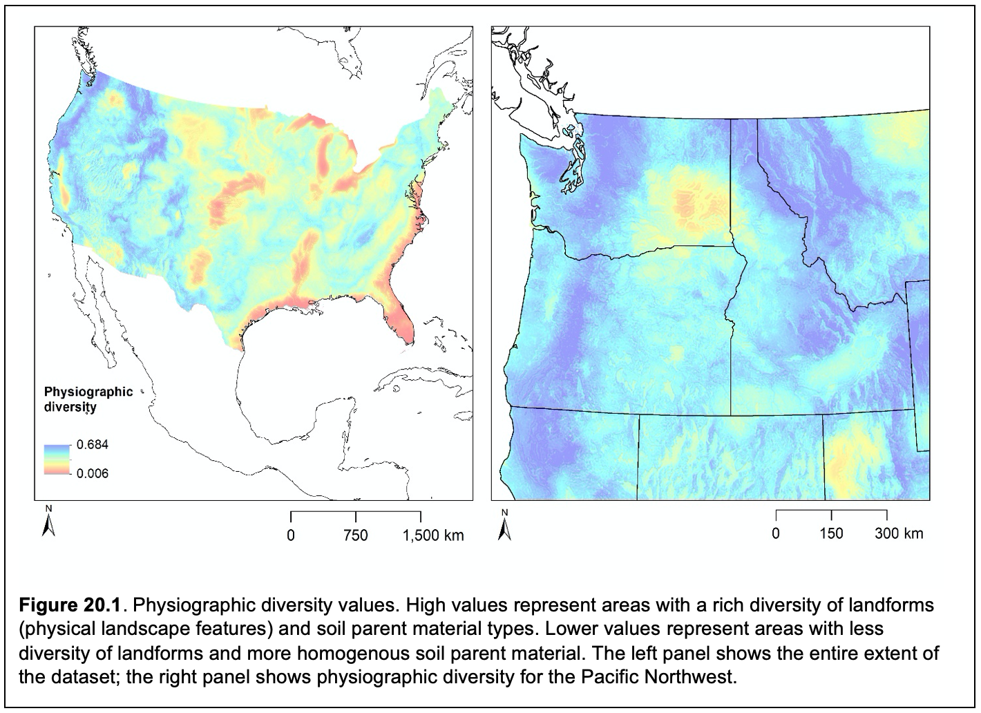
This dataset contains a set of seven data layers that depict the spatial patterns in physical features of the landscape that support ecosystems and evolutionary processes. These include landforms, continuous heat-load index, multi-scale topographic position index, lithology, physiography, physiographic diversity (figure 20.1), and topographic diversity (see chapter glossary for definitions of terms). One of the central layers is landscape physiography that is represented as a combination of landforms (e.g., mountains, slopes, valleys) and lithology. A total of 269 "physiographic units" were mapped for the continental United States by overlaying landforms and lithology and were used to map the overall diversity of physiographic units at a variety of spatial scales, ranging from >100-km radius to approximately a 1-km radius. This metric of physiographic diversity essentially represents how varied or how uniform the physical landscape is for locations throughout the United States. Mountainous areas generally have much higher physiographic diversity than flat plains, and thus may provide a greater diversity of environmental conditions for plants and animals.
Data Access: https://www.sciencebase.gov/catalog/item/564b4bb0e4b0ebfbef0d31d2
Conservation Applications
Potential conservation applications of this dataset could include the following:
- A primary application of this dataset is to guide "coarse-filter" approaches to conservation, which focus more on conserving a variety of physical features of the landscape rather than on individual species or ecosystems. Physiographic diversity was positively correlated with vertebrate species richness (Pearson correlation ~ 0.45) supporting the idea that physiographic diversity promotes biodiversity (Theobald et al., 2015). In some cases, the dataset could be adapted for "fine-filter" conservation approaches focused on individual species, e.g., by locating areas of greatest physiographic diversity within a species' range. The study that produced these datasets (Theobald et al., 2015) included a gap analysis component in which the level of land protection was assessed for each landform class. In general, landforms associated with more rugged, mountainous areas were better protected (e.g., peaks and cliffs) and lower-elevation areas were less protected (e.g., flat slopes and valley bottoms). This may point to a need to better protect some of these lower-elevation landforms in order to conserve overall landform diversity.
Applicable scales for detailed spatial assessments:
- For conservation applications requiring detailed assessment of spatial variation of the dataset within a geographic boundary (such as a protected area), the following geographic scales may be most appropriate (see appendix 3 for more information).
- At the scale of: a local watershed (12-digit hydrologic unit code [HUC-12]), a Bureau of Land Management (BLM) district, a river watershed (8-digit hydrologic unit code [HUC-8]), an individual county, a national forest, a level-3 ecoregion (e.g., the North Cascades), a single state (Washington, Oregon, or Idaho), a region (multiple states in the Pacific Northwest or in western North America), the continental United States.
Applicable scales for assessing general patterns:
- Due to spatial resolution, the dataset may not show detailed spatial variation at the following geographic scales, however, the dataset may be useful to assess general patterns or for comparison to other locations (see appendix 3 for more information).
- At the scale of: a small (< 1 km2) nature preserve, a state park or state wildlife area.
Use of the dataset in conservation applications may be limited by the following considerations:
- Because this dataset represents an abiotic "coarse-filter" approach to providing information for conservation decision-making, it focuses on the physical attributes of the landscape (the conservation "stage") rather than species (the "actors"). This dataset would likely be combined with other sources of information to enable assessment of individual species, ecosystems, or biological processes. Conservation decision-making is commonly informed by a range of considerations other than physiography, including ecological issues (e.g., endangered species, disturbances, and sensitive habitats) and pragmatic considerations (e.g., social, economic, and administrative issues).
Past or current conservation applications:
Dataset citation:
Theobald, D. M., D. Harrison-Atlas, and W. B. Monahan. 2015. Ecologically-relevant maps of landforms and physiographic diversity for climate adaptation planning. PLoS One 10:e0143619.
Dataset documentation link:
https://doi.org/10.1371/journal.pone.0143619 (open access)
Data access:
Landform maps are available in the public data catalog associated with Google Earth Engine and may be downloaded from: https://www.sciencebase.gov/catalog/item/564b4bb0e4b0ebfbef0d31d2
Physiographic diversity maps are not available for interactive online map viewing and may be obtained by contacting the corresponding author.
Metadata access:
Formal metadata is available from: https://www.sciencebase.gov/catalog/item/564b4bb0e4b0ebfbef0d31d2
Dataset corresponding author:
David Theobald
Conservation Science Partners
[email protected]
Data type category (as defined in the Introduction to this guidebook): Topoedaphic
Species or ecosystems represented: This dataset does not represent any individual species or ecosystems.
Units of mapped values: unitless; represents Shannon-Weaver diversity index
Range of mapped values: Physiographic diversity values range conceptually from 0 to 1, in practice they range from 0.006 to 0.684.
Spatial data type: a raster dataset (grid)
Data file format(s): GeoTiff (.tif)
Spatial resolution:
For landform maps: ~30 m (0.00026949459 decimal seconds)
For physiographic diversity: ~270 m
Geographic coordinate system:
For landform maps: World Geodetic System (WGS) 1984
For physiographic diversity: North American Datum of 1983
Projected coordinate system:
For landform maps: World Geodetic System (WGS) 1984
For physiographic diversity: North American Datum of 1983 Albers
Spatial extent: Conterminous United States
Dataset truncation: The dataset is truncated along the United States borders with Canada and Mexico.
Time period represented: Static (relatively unchanging over time)
Methods overview:
First, landforms were mapped using the TPI. Highly positive TPI values are associated with peaks and ridges, while highly negative TPI values are associated with valley bottoms. Landforms were further classified as "warm", "neutral", or "cool" based on a topographic metric that approximates incoming solar radiation. A national-scale dataset on lithology (Soller et al., 2009) was used to represent soil parent material and was overlaid on the landform maps to generate physiographic units. For example, areas that were classified as the "warm upper slope" landform and as "carbonate" lithology became a physiographic unit of "warm upper slope, carbonate". This overlay of landforms and lithology resulted in 269 physiographic units. Finally, the Shannon-Weaver diversity index (an index commonly used to quantify diversity of species in an area) was calculated to represent the diversity of physiographic units within an area of a given size (radius). This was done for seven radii ranging from 1.2 km to 115.8 km (Theobald et al., 2015).
This dataset relied on the following general types of models: Terrain or geomorphology models
This dataset employed the following specific models:
Topographic position index (TPI)
Modified version of the topographic heat-load index (McCune and Keon 2002)
Major input data sources for this dataset included:
Digital elevation models (DEMs) or topography, lithology (surficial materials) representing soil parent material
The mapped values of the dataset may be interpreted as follows:
For landform maps: values are categorical and represent various landform classes.
For physiographic diversity: values are continuous and unitless and represent the degree to which a given area has a strong diversity of landforms and soil parent material types. Low values for physiographic diversity are more common in flat plains or areas of homogenous lithology. High values for physiographic diversity are more common in rugged mountains or areas of highly varied lithology.
Representations of key concepts in climate-change ecology:
Landscape areas with relatively high physiographic diversity may exhibit higher adaptive capacity in the face of climate change than other areas because the diversity of nearby microclimates may enable species to seek refugia or shift their habitats to take advantage of locally favorable conditions. This increased adaptive capacity could result in reduced climate vulnerability in areas of high physiographic diversity. Note that this dataset does not represent climate exposure in that no future climate projections were used.
As described in chapter 19, conservation of areas with relatively high physiographic diversity may be part of a “coarse-filter” approach to biodiversity conservation under climate change, consistent with the idea of “conserving nature’s stage” (Beier et al., 2015). This approach can be combined with more “fine-filter” approaches that also incorporate information about individual species or groups of species.
This dataset involves the following assumptions, simplifications, and caveats:
Although physiographic diversity was calculated at a range of scales, very fine-scale (e.g., meter-scale or sub-meter-scale) diversity of microclimates was not captured. Inputs to this analysis were topographic and lithologic. Thus, physiographic diversity does not incorporate other possible physical features and processes that could affect ecosystems, such as groundwater expression (e.g., in springs or seeps) and orographic effects (e.g., rain shadows). The model of continuous HLI assumes insolation reflecting the sun at noon on the equinox.
Quantification of uncertainty:
This dataset does not include any quantification of uncertainty relating to the mapped values.
Field verification:
Field verification of this dataset was not performed, however, classification of certain landforms (cliffs and flats) was checked against geomorphological types from the Soil Survey Geographic Database (SSURGO) (Natural Resource Conservation Service, 2014).
Prior to dataset publication, peer review was conducted by external review (at least two anonymous reviewers, each from a different institution).
Beier, P., M. L. Hunter, and M. Anderson. 2015. Special section: conserving nature’s stage. Conservation Biology 29:613–617.
Jenness, J. 2006. Topographic position index (tip_jen.avx) extension for ArcView 3.x.
McCune, B., and D. Keon. 2002. Equations for potential annual direct incident radiation and heat load. Journal of Vegetation Science 13:603–606.
Natural Resource Conservation Service. 2014. Soil Survey Geographic (SSURGO) Database. http://sdmdataaccess.nrcs.usda.gov/.
Soller, D., M. Reheis, C. Garrity, and D. Van Sistine. 2009. Map database for surficial materials in the conterminous United States. U.S. Geological Survey Data Series 425.
Theobald, D. M., D. Harrison-atlas, and W. B. Monahan. 2015. Ecologically-relevant maps of landforms and physiographic diversity for climate adaptation planning. PLoS One 10:e0143619.